In this article we will look to build a collaberitive filtering model from scratch, using pure Pytorch and some support from the Fastai deep learning library.
In this article we will look to build a collaberitive filtering model from scratch, using pure Pytorch and some support from the Fastai deep learning library. We will also look at the theory and mathematics behind collaberative filtering.
2 Dataset
We will use the MovieLens dataset, and a special subset curated by fastai of the 100,000 movies. This consists of 2 separate tables for ratings and movies, which we will join together.
The key data here is the ratings i.e. the user-movie ratings, as we can see in the listing above. In collaberative filtering, an easier way to see this is as a user-item matrix, with movies as columns, users as rows, and cells as the ratings for each user-movie combination.
We can see here some cells are not filled in which are ratings we do not know, these are the values we would like to predict so we can know for each user which movie they would like.
So how might we approach this? If we imagine there are some reasons that effect peoples preferences, lets call them factors such as genre, actors etc then that might give us a basis to figure out which users would like each movie. What if we could represent these factors as a set of numbers? then we could represent each user and movie as a unique set of these numbers (or vectors) representing how much of each of the factors that user or movie represented.
Then we could say, we want each of these user and movie factors vectors when multipled to equal a rating. This would give us a basis to learn these factors, as we have ratings we know, and we could use these to estimate the ratings we don’t know. This approach of using movie vectors multipled by user vectors and summed up is known as the dot product and is the basis of matrix multiplication.
So we can randomly initialise these user and movie vectors, and learn the correct values for these that predict the ratings we know, using gradient descent.
So to do the dot product we could look up the index of each user and movie, then multiply the vectors. But neural networks don’t know how to look up using an index, they only multiply matrices together. However we can do a index looking up using matrix multiplication by using one-hot encoded vectors.
The matrix you index by multiplying by a one-hot encoded matrix, is called an embedding or embedding matrix. So our model will learn the values of these embedding matrices for the users and movies, using gradient descent.
It’s actually very easy to create a collaberative filtering model using fastai’s higher level methods - but we are going to explore doing this from scratch in this article.
We will now create our first collaberative filtering model from scratch. This will contain the embedding matrices for the users and movies, and will implement a method (in Pytorch this is normally the forward method) to do a dot product of these 2 matrices.
So the number of factors for each user and movie matrix will be determined when the model is initialised.
class DotProduct(Module):def__init__(self, n_users, n_movies, n_factors):self.user_factors = Embedding(n_users, n_factors)self.movie_factors = Embedding(n_movies, n_factors)def forward(self, x): users =self.user_factors(x[:,0]) movies =self.movie_factors(x[:,1])return (users * movies).sum(dim=1)
So the input x to the model will be a tensor of whatever the batch size is multiplied by 2 - where the first column (x[:, 0]) contains the user IDs and the second column (x[:, 1]) contains the movie IDs. So the input essentially has 2 columns.
x,y = dls.one_batch()x.shape
torch.Size([64, 2])
So we have defined our architecture and so can now create a learner to optimise the model. Because we are building the model from scratch we will use the Learner class to do this. We will use MSE as our loss function as this is a regression problem i.e. we are predicting a number, the rating.
n_users =len(dls.classes['user'])n_movies =len(dls.classes['title'])# Create model with 50 factors for users and movies eachmodel = DotProduct(n_users, n_movies, 50)# Create Learner objectlearn = Learner(dls, model, loss_func=MSELossFlat())
# Train modellearn.fit_one_cycle(5, 5e-3)
epoch
train_loss
valid_loss
time
0
1.336391
1.275613
00:09
1
1.111210
1.126141
00:09
2
0.988222
1.014545
00:09
3
0.844100
0.912820
00:09
4
0.813798
0.898948
00:09
5 Collaberative filtering - Model 2
So how can we improve the model? we know the predictions - the ratings: should be between 0-5. Perhaps we can help our model by ensuring the predictions are forced between these valid values? We can use a sigmoid function to do this.
model = DotProduct(n_users, n_movies, 50)learn = Learner(dls, model, loss_func=MSELossFlat())learn.fit_one_cycle(5, 5e-3)
epoch
train_loss
valid_loss
time
0
0.985542
1.002896
00:10
1
0.869398
0.914294
00:10
2
0.673619
0.873486
00:10
3
0.480611
0.878555
00:10
4
0.381930
0.882388
00:10
6 Collaberative filtering - Model 3
So while that didn’t make a huge difference, there is more we can do to improve. At the moment by using our user and movie embedding matrices, this only gives us a sense of how a particular movie or user is described as specific values for these latent factors. What we don’t have is a way to indicate something general about a particular movie or user such as this person is really fussy, or this movie is generally good or not good.
We can encode this general skew for each movie and user by including a bias value for each, which we can add after we have done the dot product. So lets add bias to our model.
class DotProductBias(Module):def__init__(self, n_users, n_movies, n_factors, y_range=(0,5.5)):self.user_factors = Embedding(n_users, n_factors)self.user_bias = Embedding(n_users, 1)self.movie_factors = Embedding(n_movies, n_factors)self.movie_bias = Embedding(n_movies, 1)self.y_range = y_rangedef forward(self, x): users =self.user_factors(x[:,0]) movies =self.movie_factors(x[:,1]) res = (users * movies).sum(dim=1, keepdim=True) res +=self.user_bias(x[:,0]) +self.movie_bias(x[:,1])return sigmoid_range(res, *self.y_range)
model = DotProductBias(n_users, n_movies, 50)learn = Learner(dls, model, loss_func=MSELossFlat())learn.fit_one_cycle(5, 5e-3)
epoch
train_loss
valid_loss
time
0
0.941588
0.955934
00:10
1
0.844541
0.865852
00:10
2
0.603601
0.862635
00:10
3
0.420309
0.883469
00:10
4
0.293037
0.890913
00:10
So this started much better, but then got worse! Why is this? This looks like a case of overfitting. So we can’t use data augmentation for this type of model, so we need some other way to stop the model fitting too much to the data i.e. some kind of regularization. One way to do this is with weight decay
7 Weight decay
So with weight decay, aka L2 regularization - adds an extra term to the loss function as the sum of all the weights squared. This will penalise our model for getting more complex than it needs to be i.e. overfitting, so this will encorage our model to have weights as small as possible the get the job done i.e. occams razor.
Why weights squared? The idea is the larger the model parameters are, the steeper the slope of the loss function. This can cause the model to focus too much on the data points in the training set. Adding weight decay will make training harder, but will force our model to be as simple as possible, less able to memorise the training data - and force it to generalise better.
Rather than calculate the sum of all weights squared, we take the derivative which is 2 x parameters and addd to our loss e.g.
parameters.grad += wd * 2 * parameters
Where wd is a factor we can control.
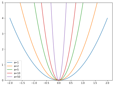
x = np.linspace(-2,2,100)a_s = [1,2,5,10,50] ys = [a * x**2for a in a_s]_,ax = plt.subplots(figsize=(8,6))for a,y inzip(a_s,ys): ax.plot(x,y, label=f'a={a}')ax.set_ylim([0,5])ax.legend();
So we used a pre-made Embeddings class to make our embedding matrices, but did’nt see how it works so lets make our own now. So we need a randomly initialised weight matrix for each. By default Pytorch tensors are not added as trainable parameters (think why, data are tensors also) so we need to create it in a particular way to make the embeddings trainable, using the nn.Parameter class.
# # Create tensor as parameter function, with random initialisationdef create_params(size):return nn.Parameter(torch.zeros(*size).normal_(0, 0.01))# Create model with our manually created embeddingsclass DotProductBias(Module):def__init__(self, n_users, n_movies, n_factors, y_range=(0,5.5)):self.user_factors = create_params([n_users, n_factors])self.user_bias = create_params([n_users])self.movie_factors = create_params([n_movies, n_factors])self.movie_bias = create_params([n_movies])self.y_range = y_rangedef forward(self, x): users =self.user_factors[x[:,0]] movies =self.movie_factors[x[:,1]] res = (users*movies).sum(dim=1) res +=self.user_bias[x[:,0]] +self.movie_bias[x[:,1]]return sigmoid_range(res, *self.y_range)
Our models developed so far are not deep learining models, as they dont have many layers. To turn this into a deep learning model we need to take the results of the embedding lookup and concatenate those activations together - this will then give us instead a matrix that we can then pass through linear layers with activation functions (non-linearities) as we would in a deep learning model.
As we are concatinating embeddings rather than taking their dot product, the embedding matrices can have different sizes. Fastai has a handy function for reccomending optimal embedding sizes from the data.
Fastai lets you create a deep learning version of the model like this with the higher level function calls by passing use_nn=True and lets you easily create more layers e.g. here with two hidden layers, of size 100 and 50, respectively.