Medical Diagnosis of 14 Diseases Using Chest X-Rays

1 Introduction

In an earlier project I developed a deep learning model that could detect and diagnose Pneumonia from Chest X-Rays. In this project we will explore medical image diagnosis further by building a state-of-the-art chest X-ray classifier using Keras that can classify and diagnose 14 different diseases.

In particular, we will: - Pre-process and prepare a real-world X-ray dataset. - Use transfer learning to retrain a DenseNet model for X-ray image classification. - Learn a technique to handle class imbalance - Measure diagnostic performance by computing the AUC (Area Under the Curve) for the ROC (Receiver Operating Characteristic) curve. - Visualize model activity using GradCAMs.

In completing this project we will cover the following key topics in the use of deep learning in medical diagnosis:

• Data preparation
  • Visualizing data.
  • Preventing data leakage.
• Model Development
  • Addressing class imbalance.
  • Leveraging pre-trained models using transfer learning.
• Evaluation
  • AUC and ROC curves.

2 Load the Datasets

I will be using the ChestX-ray8 dataset which contains 108,948 frontal-view X-ray images of 32,717 unique patients.

• Each image in the data set contains multiple text-mined labels identifying 14 different pathological conditions.
• These in turn can be used by physicians to diagnose 8 different diseases.
• We will use this data to develop a single model that will provide binary classification predictions for each of the 14 labeled pathologies.
• In other words it will predict ‘positive’ or ‘negative’ for each of the pathologies.

You can download the entire dataset for free here.

We have taken a subset of these images of around 1000 for the purposes of this project.

This dataset has been annotated by consensus among four different radiologists for 5 of our 14 pathologies: - Consolidation - Edema - Effusion - Cardiomegaly - Atelectasis

### Loading the Data

train_df = pd.read_csv("data/nih/train-small.csv")
valid_df = pd.read_csv("data/nih/valid-small.csv")

test_df = pd.read_csv("data/nih/test.csv")

train_df.head()

	Image	Atelectasis	Cardiomegaly	Consolidation	Edema	Effusion	Emphysema	Fibrosis	Hernia	Infiltration	Mass	Nodule	PatientId	Pleural_Thickening	Pneumonia	Pneumothorax
0	00008270_015.png	0	0	0	0	0	0	0	0	0	0	0	8270	0	0	0
1	00029855_001.png	1	0	0	0	1	0	0	0	1	0	0	29855	0	0	0
2	00001297_000.png	0	0	0	0	0	0	0	0	0	0	0	1297	1	0	0
3	00012359_002.png	0	0	0	0	0	0	0	0	0	0	0	12359	0	0	0
4	00017951_001.png	0	0	0	0	0	0	0	0	1	0	0	17951	0	0	0

labels = ['Cardiomegaly', 
          'Emphysema', 
          'Effusion', 
          'Hernia', 
          'Infiltration', 
          'Mass', 
          'Nodule', 
          'Atelectasis',
          'Pneumothorax',
          'Pleural_Thickening', 
          'Pneumonia', 
          'Fibrosis', 
          'Edema', 
          'Consolidation']

### Preventing Data Leakage It is worth noting that our dataset contains multiple images for each patient. This could be the case, for example, when a patient has taken multiple X-ray images at different times during their hospital visits. In our data splitting, we have ensured that the split is done on the patient level so that there is no data “leakage” between the train, validation, and test datasets.

### Check for Leakage

We will write a function to check whether there is leakage between two datasets. We’ll use this to make sure there are no patients in the test set that are also present in either the train or validation sets.

def check_for_leakage(df1, df2, patient_col):
    """
    Return True if there any patients are in both df1 and df2.

    Args:
        df1 (dataframe): dataframe describing first dataset
        df2 (dataframe): dataframe describing second dataset
        patient_col (str): string name of column with patient IDs
    
    Returns:
        leakage (bool): True if there is leakage, otherwise False
    """
    
    # Extract patient id's for df1
    ids_df1 = df1[patient_col].values
    # Extract patient id's for df2
    ids_df2 = df2[patient_col].values
    
    # Create sets for both 
    df1_patients_unique = set(ids_df1)
    df2_patients_unique = set(ids_df2)
    
    # Find the interesction of sets 
    patients_in_both_groups = list(df1_patients_unique.intersection(df2_patients_unique))

    # If non empty then we have patients in both df
    if len(patients_in_both_groups) > 0:
        leakage = True
    else:
        leakage = False
     
    return leakage

# Run test
check_for_leakage_test(check_for_leakage)

Test Case 1

df1
   patient_id
0           0
1           1
2           2
df2
   patient_id
0           2
1           3
2           4
leakage output: True 
-------------------------------------
Test Case 2

df1
   patient_id
0           0
1           1
2           2
df2
   patient_id
0           3
1           4
2           5
leakage output: False 

 All tests passed.

Expected output

Test Case 1

df1
   patient_id
0           0
1           1
2           2
df2
   patient_id
0           2
1           3
2           4
leakage output: True 
-------------------------------------
Test Case 2

df1
   patient_id
0           0
1           1
2           2
df2
   patient_id
0           3
1           4
2           5
leakage output: False

 All tests passed.

print("leakage between train and valid: {}".format(check_for_leakage(train_df, valid_df, 'PatientId')))
print("leakage between train and test: {}".format(check_for_leakage(train_df, test_df, 'PatientId')))
print("leakage between valid and test: {}".format(check_for_leakage(valid_df, test_df, 'PatientId')))

leakage between train and valid: True
leakage between train and test: False
leakage between valid and test: False

Expected output

leakage between train and valid: True
leakage between train and test: False
leakage between valid and test: False

### Preparing Images

With our dataset splits ready, we can now proceed with setting up our model to consume them. - For this we will use the off-the-shelf ImageDataGenerator class from the Keras framework, which allows us to build a “generator” for images specified in a dataframe. - This class also provides support for basic data augmentation such as random horizontal flipping of images. - We also use the generator to transform the values in each batch so that their mean is \(0\) and their standard deviation is 1. - This will facilitate model training by standardizing the input distribution. - The generator also converts our single channel X-ray images (gray-scale) to a three-channel format by repeating the values in the image across all channels. - We will want this because the pre-trained model that we’ll use requires three-channel inputs.

def get_train_generator(df, image_dir, x_col, y_cols, shuffle=True, batch_size=8, seed=1, target_w = 320, target_h = 320):
    """
    Return generator for training set, normalizing using batch
    statistics.

    Args:
      train_df (dataframe): dataframe specifying training data.
      image_dir (str): directory where image files are held.
      x_col (str): name of column in df that holds filenames.
      y_cols (list): list of strings that hold y labels for images.
      batch_size (int): images per batch to be fed into model during training.
      seed (int): random seed.
      target_w (int): final width of input images.
      target_h (int): final height of input images.
    
    Returns:
        train_generator (DataFrameIterator): iterator over training set
    """        
    print("getting train generator...") 
    # normalize images
    image_generator = ImageDataGenerator(
        samplewise_center=True,
        samplewise_std_normalization= True)
    
    # flow from directory with specified batch size
    # and target image size
    generator = image_generator.flow_from_dataframe(
            dataframe=df,
            directory=image_dir,
            x_col=x_col,
            y_col=y_cols,
            class_mode="raw",
            batch_size=batch_size,
            shuffle=shuffle,
            seed=seed,
            target_size=(target_w,target_h))
    
    return generator

Build a separate generator for valid and test sets

Now we need to build a new generator for validation and testing data.

Why can’t we use the same generator as for the training data?

Look back at the generator we wrote for the training data. - It normalizes each image per batch, meaning that it uses batch statistics. - We should not do this with the test and validation data, since in a real life scenario we don’t process incoming images a batch at a time (we process one image at a time). - Knowing the average per batch of test data would effectively give our model an advantage.
- The model should not have any information about the test data.

What we need to do is normalize incoming test data using the statistics computed from the training set. * We implement this in the function below. * There is one technical note. Ideally, we would want to compute our sample mean and standard deviation using the entire training set. * However, since this is extremely large, that would be very time consuming. * In the interest of time, we’ll take a random sample of the dataset and calcualte the sample mean and sample standard deviation.

def get_test_and_valid_generator(valid_df, test_df, train_df, image_dir, x_col, y_cols, sample_size=100, batch_size=8, seed=1, target_w = 320, target_h = 320):
    """
    Return generator for validation set and test set using 
    normalization statistics from training set.

    Args:
      valid_df (dataframe): dataframe specifying validation data.
      test_df (dataframe): dataframe specifying test data.
      train_df (dataframe): dataframe specifying training data.
      image_dir (str): directory where image files are held.
      x_col (str): name of column in df that holds filenames.
      y_cols (list): list of strings that hold y labels for images.
      sample_size (int): size of sample to use for normalization statistics.
      batch_size (int): images per batch to be fed into model during training.
      seed (int): random seed.
      target_w (int): final width of input images.
      target_h (int): final height of input images.
    
    Returns:
        test_generator (DataFrameIterator) and valid_generator: iterators over test set and validation set respectively
    """
    print("getting train and valid generators...")
    # get generator to sample dataset
    raw_train_generator = ImageDataGenerator().flow_from_dataframe(
        dataframe=train_df, 
        directory=IMAGE_DIR, 
        x_col="Image", 
        y_col=labels, 
        class_mode="raw", 
        batch_size=sample_size, 
        shuffle=True, 
        target_size=(target_w, target_h))
    
    # get data sample
    batch = raw_train_generator.next()
    data_sample = batch[0]

    # use sample to fit mean and std for test set generator
    image_generator = ImageDataGenerator(
        featurewise_center=True,
        featurewise_std_normalization= True)
    
    # fit generator to sample from training data
    image_generator.fit(data_sample)

    # get test generator
    valid_generator = image_generator.flow_from_dataframe(
            dataframe=valid_df,
            directory=image_dir,
            x_col=x_col,
            y_col=y_cols,
            class_mode="raw",
            batch_size=batch_size,
            shuffle=False,
            seed=seed,
            target_size=(target_w,target_h))

    test_generator = image_generator.flow_from_dataframe(
            dataframe=test_df,
            directory=image_dir,
            x_col=x_col,
            y_col=y_cols,
            class_mode="raw",
            batch_size=batch_size,
            shuffle=False,
            seed=seed,
            target_size=(target_w,target_h))
    return valid_generator, test_generator

With our generator function ready, let’s make one generator for our training data and one each of our test and validation datasets.

IMAGE_DIR = "data/nih/images-small/"
train_generator = get_train_generator(train_df, IMAGE_DIR, "Image", labels)
valid_generator, test_generator= get_test_and_valid_generator(valid_df, test_df, train_df, IMAGE_DIR, "Image", labels)

getting train generator...
Found 1000 validated image filenames.
getting train and valid generators...
Found 1000 validated image filenames.
Found 200 validated image filenames.
Found 420 validated image filenames.

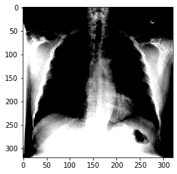
Let’s peek into what the generator gives our model during training and validation. We can do this by calling the __get_item__(index) function:

x, y = train_generator.__getitem__(0)
plt.imshow(x[0]);

Clipping input data to the valid range for imshow with RGB data ([0..1] for floats or [0..255] for integers).

## Model Development

Now we’ll move on to model training and development. We have a few practical challenges to deal with before actually training a neural network, though. The first is class imbalance.

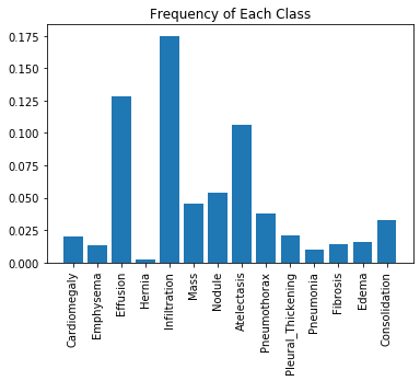
### Addressing Class Imbalance One of the challenges with working with medical diagnostic datasets is the large class imbalance present in such datasets. Let’s plot the frequency of each of the labels in our dataset:

plt.xticks(rotation=90)
plt.bar(x=labels, height=np.mean(train_generator.labels, axis=0))
plt.title("Frequency of Each Class")
plt.show()

We can see from this plot that the prevalance of positive cases varies significantly across the different pathologies. (These trends mirror the ones in the full dataset as well.) * The Hernia pathology has the greatest imbalance with the proportion of positive training cases being about 0.2%. * But even the Infiltration pathology, which has the least amount of imbalance, has only 17.5% of the training cases labelled positive.

Ideally, we would train our model using an evenly balanced dataset so that the positive and negative training cases would contribute equally to the loss.

If we use a normal cross-entropy loss function with a highly unbalanced dataset, as we are seeing here, then the algorithm will be incentivized to prioritize the majority class (i.e negative in our case), since it contributes more to the loss.

Impact of class imbalance on loss function

Let’s take a closer look at this. Assume we would have used a normal cross-entropy loss for each pathology. We recall that the cross-entropy loss contribution from the \(i^{th}\) training data case is:

\[\mathcal{L}_{cross-entropy}(x_i) = -(y_i \log(f(x_i)) + (1-y_i) \log(1-f(x_i))),\]

where \(x_i\) and \(y_i\) are the input features and the label, and \(f(x_i)\) is the output of the model, i.e. the probability that it is positive.

Note that for any training case, either \(y_i=0\) or else \((1-y_i)=0\), so only one of these terms contributes to the loss (the other term is multiplied by zero, and becomes zero).

We can rewrite the overall average cross-entropy loss over the entire training set \(\mathcal{D}\) of size \(N\) as follows:

\[\mathcal{L}_{cross-entropy}(\mathcal{D}) = - \frac{1}{N}\big( \sum_{\text{positive examples}} \log (f(x_i)) + \sum_{\text{negative examples}} \log(1-f(x_i)) \big).\]

Using this formulation, we can see that if there is a large imbalance with very few positive training cases, for example, then the loss will be dominated by the negative class. Summing the contribution over all the training cases for each class (i.e. pathological condition), we see that the contribution of each class (i.e. positive or negative) is:

\[freq_{p} = \frac{\text{number of positive examples}}{N} \]

\[\text{and}\]

\[freq_{n} = \frac{\text{number of negative examples}}{N}.\]

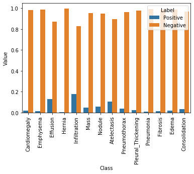
### Compute Class Frequencies Let’s write a function to calculate these frequences for each label in our dataset.

def compute_class_freqs(labels):
    """
    Compute positive and negative frequences for each class.

    Args:
        labels (np.array): matrix of labels, size (num_examples, num_classes)
    Returns:
        positive_frequencies (np.array): array of positive frequences for each
                                         class, size (num_classes)
        negative_frequencies (np.array): array of negative frequences for each
                                         class, size (num_classes)
    """
    
    # total number of patients (rows)
    N = labels.shape[0]
    
    positive_frequencies = np.sum(labels, axis=0) / N
    negative_frequencies = 1 - positive_frequencies

    return positive_frequencies, negative_frequencies

### Compute frequencies     
compute_class_freqs_test(compute_class_freqs)

Labels:
[[1 0 0]
 [0 1 1]
 [1 0 1]
 [1 1 1]
 [1 0 1]]

Pos Freqs:  [0.8 0.4 0.8]
Neg Freqs:  [0.2 0.6 0.2] 

 All tests passed.

Expected output

Labels:
[[1 0 0]
 [0 1 1]
 [1 0 1]
 [1 1 1]
 [1 0 1]]

Pos Freqs:  [0.8 0.4 0.8]
Neg Freqs:  [0.2 0.6 0.2] 

 All tests passed. 

Now we’ll compute frequencies for our training data.

freq_pos, freq_neg = compute_class_freqs(train_generator.labels)
freq_pos

array([0.02 , 0.013, 0.128, 0.002, 0.175, 0.045, 0.054, 0.106, 0.038,
       0.021, 0.01 , 0.014, 0.016, 0.033])

Expected output

array([0.02 , 0.013, 0.128, 0.002, 0.175, 0.045, 0.054, 0.106, 0.038,
       0.021, 0.01 , 0.014, 0.016, 0.033])

Let’s visualize these two contribution ratios next to each other for each of the pathologies:

data = pd.DataFrame({"Class": labels, "Label": "Positive", "Value": freq_pos})
data = data.append([{"Class": labels[l], "Label": "Negative", "Value": v} for l,v in enumerate(freq_neg)], ignore_index=True)
plt.xticks(rotation=90)
f = sns.barplot(x="Class", y="Value", hue="Label" ,data=data)

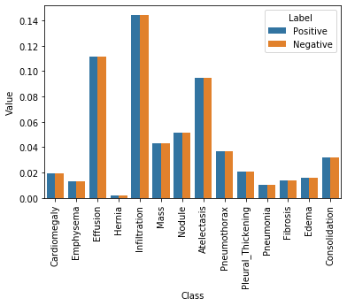
As we see in the above plot, the contributions of positive cases is significantly lower than that of the negative ones. However, we want the contributions to be equal. One way of doing this is by multiplying each example from each class by a class-specific weight factor, \(w_{pos}\) and \(w_{neg}\), so that the overall contribution of each class is the same.

To have this, we want

\[w_{pos} \times freq_{p} = w_{neg} \times freq_{n},\]

which we can do simply by taking

\[w_{pos} = freq_{neg}\] \[w_{neg} = freq_{pos}\]

This way, we will be balancing the contribution of positive and negative labels.

pos_weights = freq_neg
neg_weights = freq_pos
pos_contribution = freq_pos * pos_weights 
neg_contribution = freq_neg * neg_weights

Let’s verify this by graphing the two contributions next to each other again:

data = pd.DataFrame({"Class": labels, "Label": "Positive", "Value": pos_contribution})
data = data.append([{"Class": labels[l], "Label": "Negative", "Value": v} 
                        for l,v in enumerate(neg_contribution)], ignore_index=True)
plt.xticks(rotation=90)
sns.barplot(x="Class", y="Value", hue="Label" ,data=data);

As the above figure shows, by applying these weightings the positive and negative labels within each class would have the same aggregate contribution to the loss function. Now let’s implement such a loss function.

After computing the weights, our final weighted loss for each training case will be

\[\mathcal{L}_{cross-entropy}^{w}(x) = - (w_{p} y \log(f(x)) + w_{n}(1-y) \log( 1 - f(x) ) ).\]

### Get Weighted Loss We will write a weighted_loss function to return a loss function that calculates the weighted loss for each batch. Recall that for the multi-class loss, we add up the average loss for each individual class. Note that we also want to add a small value, \(\epsilon\), to the predicted values before taking their logs. This is simply to avoid a numerical error that would otherwise occur if the predicted value happens to be zero.

def get_weighted_loss(pos_weights, neg_weights, epsilon=1e-7):
    """
    Return weighted loss function given negative weights and positive weights.

    Args:
      pos_weights (np.array): array of positive weights for each class, size (num_classes)
      neg_weights (np.array): array of negative weights for each class, size (num_classes)
    
    Returns:
      weighted_loss (function): weighted loss function
    """
    def weighted_loss(y_true, y_pred):
        """
        Return weighted loss value. 

        Args:
            y_true (Tensor): Tensor of true labels, size is (num_examples, num_classes)
            y_pred (Tensor): Tensor of predicted labels, size is (num_examples, num_classes)
        Returns:
            loss (float): overall scalar loss summed across all classes
        """
        # initialize loss to zero
        loss = 0.0

        for i in range(len(pos_weights)):
            # for each class, add average weighted loss for that class 
            loss_pos = -1 * K.mean(pos_weights[i] * 
                y_true[:, i] * 
                K.log(y_pred[:, i] + epsilon))
            loss_neg = -1 * K.mean( 
                neg_weights[i] * 
                (1 - y_true[:, i]) * 
                K.log(1 - y_pred[:, i] + epsilon))
            loss += loss_pos + loss_neg 
        return loss
    
    return weighted_loss

# test with a large epsilon in order to catch errors. 
# In order to pass the tests, set epsilon = 1
epsilon = 1

sess = K.get_session()
get_weighted_loss_test(get_weighted_loss, epsilon, sess)

y_true:
[[1. 1. 1.]
 [1. 1. 0.]
 [0. 1. 0.]
 [1. 0. 1.]]

w_p:
[0.25 0.25 0.5 ]

w_n:
[0.75 0.75 0.5 ]

y_pred_1:
[[0.7 0.7 0.7]
 [0.7 0.7 0.7]
 [0.7 0.7 0.7]
 [0.7 0.7 0.7]]

y_pred_2:
[[0.3 0.3 0.3]
 [0.3 0.3 0.3]
 [0.3 0.3 0.3]
 [0.3 0.3 0.3]]

If you weighted them correctly, you'd expect the two losses to be the same.
With epsilon = 1, your losses should be, L(y_pred_1) = -0.4956203 and L(y_pred_2) = -0.4956203

Your outputs:

L(y_pred_1) =  -0.4956203
L(y_pred_2) =  -0.4956203
Difference: L(y_pred_1) - L(y_pred_2) =  0.0 

 All tests passed.

Expected output

with epsilon = 1

Outputs:

L(y_pred_1) =  -0.4956203
L(y_pred_2) =  -0.4956203
Difference: L(y_pred_1) - L(y_pred_2) =  0.0 

 All tests passed.   

### DenseNet121

Next, we will use a pre-trained DenseNet121 model which we can load directly from Keras and then add two layers on top of it: 1. A GlobalAveragePooling2D layer to get the average of the last convolution layers from DenseNet121. 2. A Dense layer with sigmoid activation to get the prediction logits for each of our classes.

We can set our custom loss function for the model by specifying the loss parameter in the compile() function.

# create the base pre-trained model
base_model = DenseNet121(weights='models/nih/densenet.hdf5', include_top=False)

x = base_model.output

# add a global spatial average pooling layer
x = GlobalAveragePooling2D()(x)

# and a logistic layer
predictions = Dense(len(labels), activation="sigmoid")(x)

model = Model(inputs=base_model.input, outputs=predictions)
model.compile(optimizer='adam', loss=get_weighted_loss(pos_weights, neg_weights))

## Training

With our model ready for training, we could use the model.fit() function in Keras to train our model.

• We are training on a small subset of the dataset (~1%).
  
• So what we care about at this point is to make sure that the loss on the training set is decreasing.

If we were going to train this model we could use the following code to do this:

history = model.fit_generator(train_generator, 
                              validation_data=valid_generator,
                              steps_per_epoch=100, 
                              validation_steps=25, 
                              epochs = 3)

plt.plot(history.history['loss'])
plt.ylabel("loss")
plt.xlabel("epoch")
plt.title("Training Loss Curve")
plt.show()

In our case, we will alternatively load a pre-trained model.

### Training on the Larger Dataset

Given that the original dataset is 40GB+ in size and the training process on the full dataset takes a few hours, I have access to a pre-trained the model on a GPU-equipped machine which provides the weights file from our model (with a batch size of 32 instead) to be used for the rest of the project.

Let’s load our pre-trained weights into the model now:

model.load_weights("models/nih/pretrained_model.h5")

## Prediction and Evaluation

Now that we have a model, let’s evaluate it using our test set.

predicted_vals = model.predict_generator(test_generator, steps = len(test_generator))

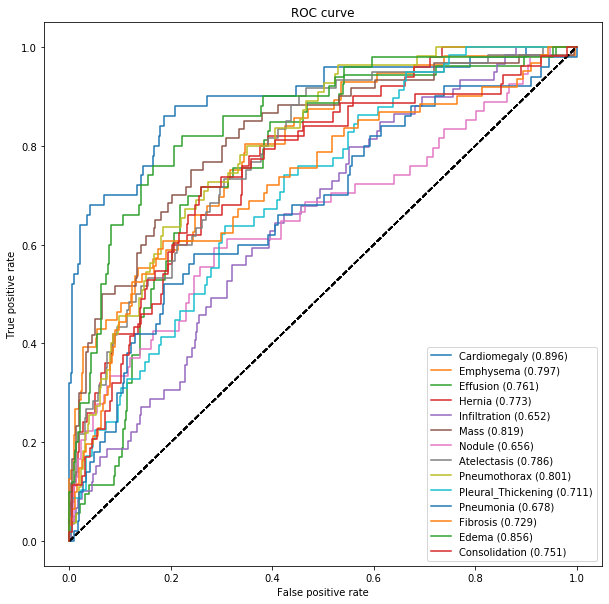
### ROC Curve and AUROC For evaluating this model we will use a metric called the AUC (Area Under the Curve) from the ROC (Receiver Operating Characteristic) curve. This is also referred to as the AUROC value.

The key insight for interpreting this plot is that a curve that the more to the left and the top has more “area” under it, this indicates that the model is performing better.

• roc_curve
• roc_auc_score

auc_rocs = util.get_roc_curve(labels, predicted_vals, test_generator)

For details about the best performing methods and their performance on this dataset, please read the following papers:

• CheXNet
• CheXpert
• ChexNeXt

### Visualizing Learning with GradCAM

One of the challenges of using deep learning in medicine is that the complex architecture used for neural networks makes them much harder to interpret compared to traditional machine learning models (e.g. linear models). There are no easily interpretable model coeffcients.

One of the most common approaches aimed at increasing the interpretability of models for computer vision tasks is to use Class Activation Maps (CAM).

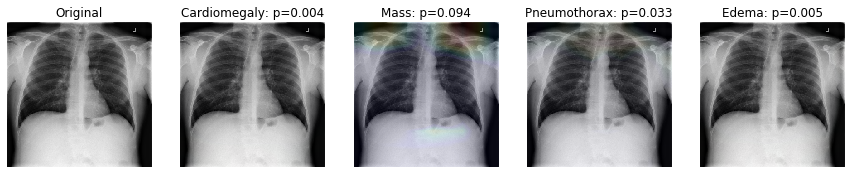
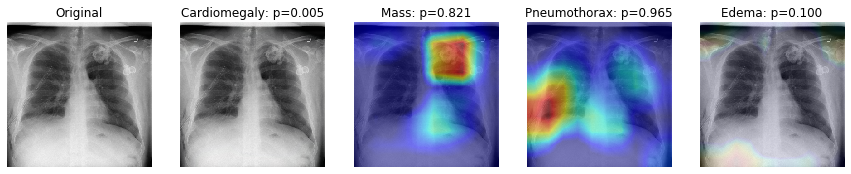
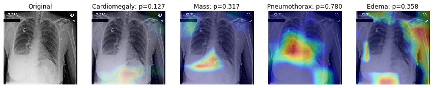
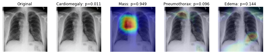
In this section we will use a GradCAM’s technique to produce a heatmap highlighting the important regions in the image for predicting the pathological condition.

This is done by extracting the gradients of each predicted class, flowing into our model’s final convolutional layer.

Indeed I used this method previously in an earlier article using fastai’s deep learning library as an alternative to Keras.

It is worth mentioning that GradCAM does not provide a full explanation of the reasoning for each classification probability. However, it is still a useful tool for “debugging” our model and augmenting our prediction so that an expert could validate that a prediction is indeed due to the model focusing on the right regions of the image.

First we will load the small training set and setup to look at the 4 classes with the highest performing AUC measures.

df = pd.read_csv("data/nih/train-small.csv")
IMAGE_DIR = "data/nih/images-small/"

# only show the labels with top 4 AUC
labels_to_show = np.take(labels, np.argsort(auc_rocs)[::-1])[:4]

Now let’s look at a few specific images.

util.compute_gradcam(model, '00008270_015.png', IMAGE_DIR, df, labels, labels_to_show)

Loading original image
Generating gradcam for class Cardiomegaly
Generating gradcam for class Mass
Generating gradcam for class Pneumothorax
Generating gradcam for class Edema

util.compute_gradcam(model, '00011355_002.png', IMAGE_DIR, df, labels, labels_to_show)

Loading original image
Generating gradcam for class Cardiomegaly
Generating gradcam for class Mass
Generating gradcam for class Pneumothorax
Generating gradcam for class Edema

util.compute_gradcam(model, '00029855_001.png', IMAGE_DIR, df, labels, labels_to_show)

Loading original image
Generating gradcam for class Cardiomegaly
Generating gradcam for class Mass
Generating gradcam for class Pneumothorax
Generating gradcam for class Edema

util.compute_gradcam(model, '00005410_000.png', IMAGE_DIR, df, labels, labels_to_show)

Loading original image
Generating gradcam for class Cardiomegaly
Generating gradcam for class Mass
Generating gradcam for class Pneumothorax
Generating gradcam for class Edema

3 Conclusion

In this project we looked at medical image diagnosis by building a state-of-the-art chest X-ray classifier using Keras.

In particular, looked at the following:

• Pre-processed and prepare a real-world X-ray dataset.
• Used transfer learning to retrain a DenseNet model for X-ray image classification.
• Learned a technique to handle class imbalance
• Measured diagnostic performance by computing the AUC (Area Under the Curve) for the ROC (Receiver Operating Characteristic) curve.
• Visualized model activity using GradCAMs.

Subscribe